Welcome to Pump fitting tools’s documentation!
Introduction
The Pump Fitting Tool is used generate the input to a pump model for use in the decision support system RTC-Tools 2. It reads user-supplied pump performance data and calculates the coefficients of polynomials that approximate the characteristics for pump power, the boundaries of the working area, and the relations to compute the shaft speed of the pump. The script can be used for rotordynamic pumps (both constant and variable speed) and screw pumps.
Input for the script and preprocessing
All the input data for the script is stored in a csv file like shown below. The following fields should be filled:
- Pump type: 0 for variable speed pumps, 1 for constant speed pumps, and 2 for screw pumps
- Reference pump speed
Nref(rpm) - The Q-H relation of the pump for shaft speed
Nref: flow rate Q (m3/s ) and head H (m) - Either power (W) or efficiency (-) for the given flow rates
These are the necessary inputs for a simple pump, the other features can be left as default.
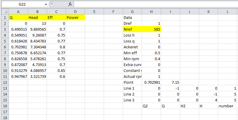
There are several extra options in the excel file:
- The loss coefficients,
Loss handLoss q, are used to specify system head lossLoss hat a specific flow rateLoss q.Ackeret: if the value is 1, then Ackeret correction is used. It can be 0 or 1.Min eff: The minimum efficiency used to bound the working area. It can vary from 0 to 1.Min rpm: The minimum pump speed fraction used to bound the working area. It can vary from 0 to 1.Actual rpm: Only used if the givenNrefis not the maximum speed. It is the ratio betweenNrefand the maximum speed. IfNrefis the maximum pump speed it can be left empty or filled with 1. (Meaning thatNrefis the 100% of the maximum speed.)Loss coef: the system losses can be given with a loss coefficient. The head losses are calculated by multiplying this coefficient with the square of the flow rate.Extra curves: Extra curves can be given to further restrict the working area. The curves can be given below, and the number of the curves should be defined here. If you use this option, then you also have to fill in the field Point. Otherwise fill in 0. Further explanation about these items can be found in section Working area selection.
Note
- The Q values should be in increasing order
- Power should reflect energy consumption, i.e. grid power (in case of an electric drive) or motor power (in case of a diesel engine drive)
- If efficiency \(\eta\) is supplied, the power P will be calculated by \(P = 9800QH/\eta\)
- Pump head H can be either static of manometric head
- If manometric head
Hmanis given, the system head losses should be specified using either (Loss q,``Loss h``) orLoss coef - If static head
Hstatis given, either the power should be supplied or the static efficiency \(H_{stat}\) based on static head i.e. \(H_{stat} = 9800QH_stat/P\) should be provided - If the static head is given, both
Loss handLoss coefshould be equal to zero.
To run the script
You can set the name of your input file in the file main.py.
43 44 45 46 47 48 49 50 51 52 53 54 55 56 57 |
    csv_file_name = 'Kuijkm_input_extrap'
    csv_file_name = 'Pannerling_input_extrap'
    #csv_file_name = 'Pannerling_input'
    #csv_file_name = 'Kuijkm_input'
    #csv_file_name = 'ExampleHomePage'
    #csv_file_name = 'Beuningen1_input_extrap'  #This is a constant speed pump
    #csv_file_name = 'buma1'

    linear = 0

    #This function reads the variables from the csv
    P, E, Q, Hread, dref, N, losshref, lossqref, minimum_efficiency, minimum_rpm, point_coordinates, ackeret_correction, extra_line_coef, pump_type, loss_coefficient, maximum_rpm, maximum_calc_rpm, constant_head = _csv_reader(csv_file_name)

    #This function removes the losses if they are expressed in Q and H
|
How to find the input data?
There are four kinds of data needed to run the script. All can be read from the pump curves.
1. Pump type
The type of pump should be specified. This information is given in the documentation of the pump.
2. Q-H relations
The Q-H relations can be read from a pump curve. A pump system curve contains the flow rate-head relations for a certain shaft speed. There might be more curves for different speeds. For this program, we need the curve belonging to the maximum speed. The head might be the static head or manometric head. Or it is also possible that both curves are given. In case the power is given later, it does not have much effect which curve is read. It is recommended to read the static head curve, as it is already corrected for the system losses. If only the manometric head curve is given, the losses can be approximated as described in the following section. In case the power is not given, then the efficiency curve should be read. Make sure that values for head and efficiency are consistent i.e. power P should follow from \(P = 9800.Q.H/\eta\).
3. Pump speed
This is the speed corresponding to the system curve read in point 2. Often the data is located on the drawing itself. Give the value in rpm.
4. Power or efficiency
Either the power or the efficiency should be given. If both are available, it is recommended to give the power. The advantage is that then the static head can be used and the static efficiency can directly obtained.
Approximation of the losses
The manometric head (\(H_{man}\)) of a pump is a measure of the pressure difference across the pump, from inlet to outlet flange. Part of this pressure is required to overcome the frictional losses in the piping system, and the remainder is used to maintain the water level difference across the pumping station – the so-called static head (\(H_{stat}\)). Thus, the static head is always lower than the manometric head and is calculated by
Head losses for a given system depend on flow rate. It is assumed here that head losses vary with flow rate squared.
There are three possible ways to account for the losses:
by specifying a loss coefficient C
\[H_{stat}= H_{man} - C Q^2\]by specifying a known head loss (\(H_{loss}\)) for certain flow rate (\(Q_{loss}\)). For any flow rate Q, the relation between static and manometric head reads
\[H_{stat}= H_{man} - H_{loss} (Q/Q_{loss})^2\]where Hmanometric is the resulting head that the pump has to overcome.
If head loss correction is used, the program is already reading the compensated heads.
- by reading directly the static head curve.
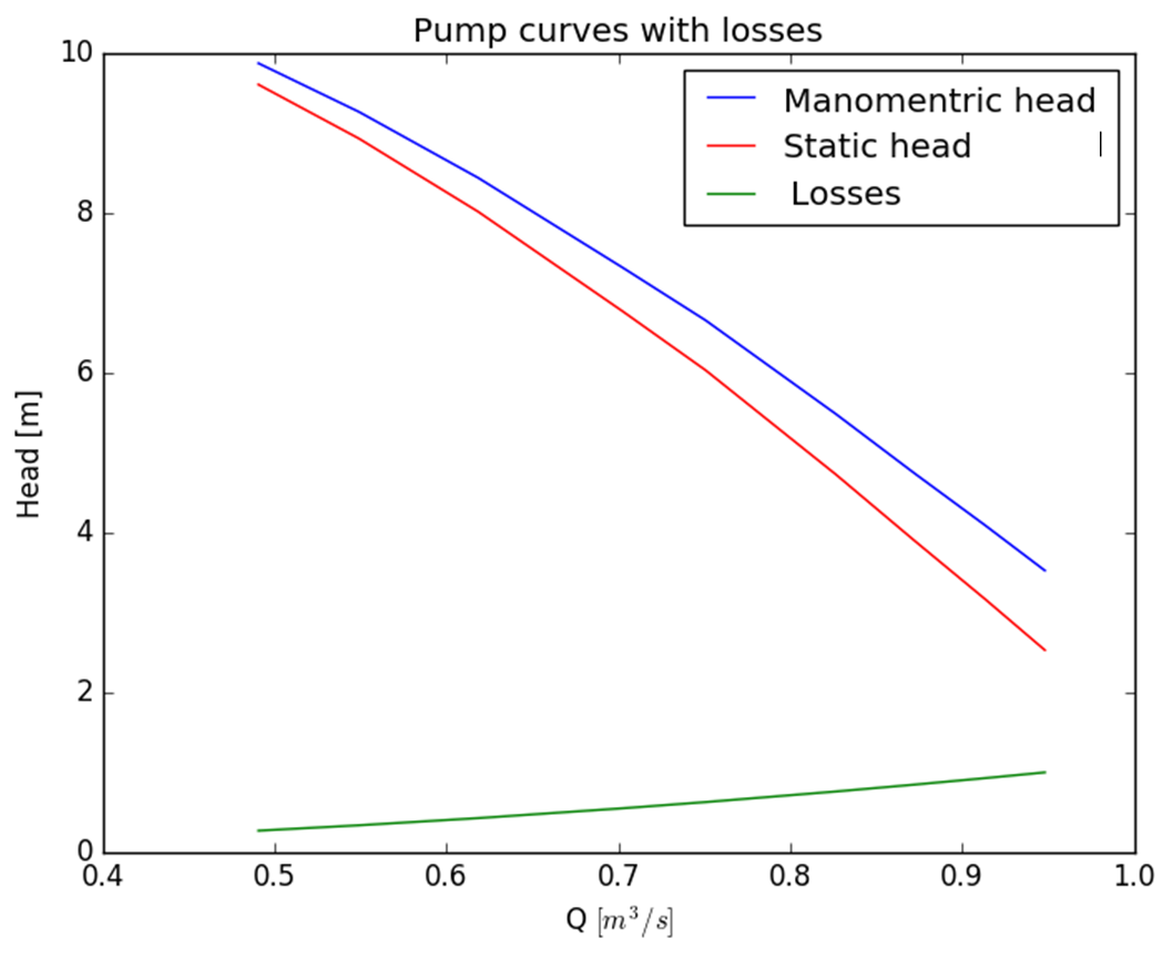
In the figure below a case with loss coefficient C=10 is plotted. It can be seen that the losses increase quadratically with flow rate.
Note
See if your data is given as static head or as manometric head.
Ackeret correction
The (manometric) efficiency of the pump is provided for a single shaft speed, either directly or through the power curve. For a variable speed pump, the efficiency would decrease with decreasing shaft speed due to a changing Reynolds number. The Ackeret correction is used to take this into account:
where (\(E_{ref}\)) is the original and (\(E\)) is the corrected efficiency. \(\alpha\) is the Ackeret parameter and its value is taken to be 0.15. \(N_{ref}\) and \(N\) are the original and the new pump speed respectively. The efficiency is bounded by 0 and 1. After this correction the power is also re-calculated. The reason is that the script (and the optimization) is working with the minimization of the power instead of efficiency.
Working area selection
The working area is bounded by the minimum and maximum shaft speed curves, and the minimum efficiency curves. These four curves are always present in case of variable speed and constant speed pumps. The exception is the screw pump. Additionally, the user can define additional curves (e.g. NPSH) that further restrict the working area. In case of additional curves, the user should also provide the coordinates of a point that is inside the working area.
Constant speed pumps
The basic four curves are used to select the working area. However, as there is only one shaft speed, there will be one curve instead of an area. This curve will be approximated with a straight line. In the input file the pump type should be set to constant speed pumps.
Screw pumps
It is possible to use to model screw pumps with this software package. In the input file the pump type should be set to screw pumps.
How does pump-fitting tools work?
The pump power is approximated with a second order convex function.
The efficiency is calculated as:
- After calculation the losses and applying the Ackeret correction,
- the power surface is obtained by using the affinity laws:
Step by step example
1. The available data
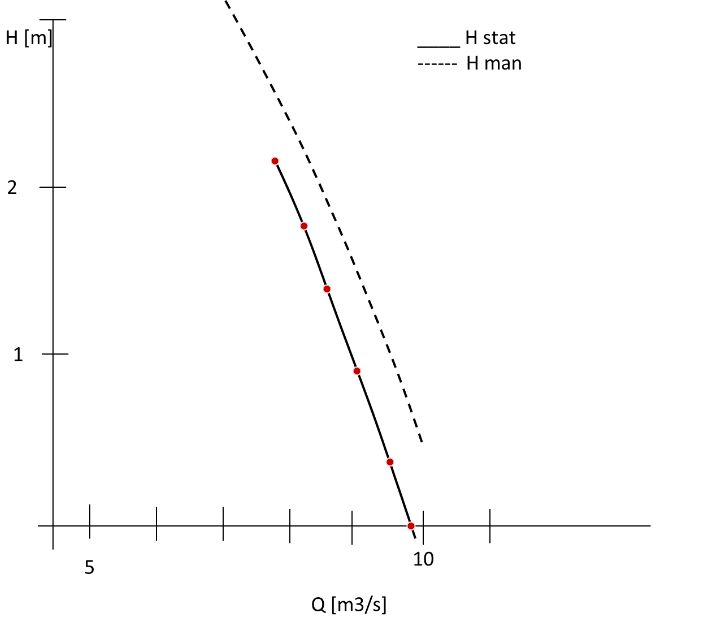
Suppose there is a variable speed pump. The following pump curves are given corresponding to 120.2 rpm. The first figure show the head curves
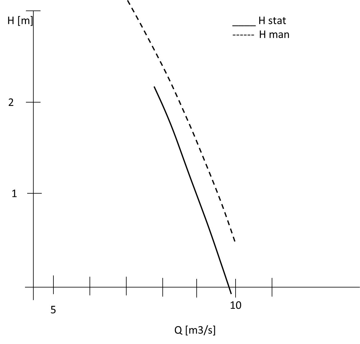
and the second one shows the power and the efficiency.
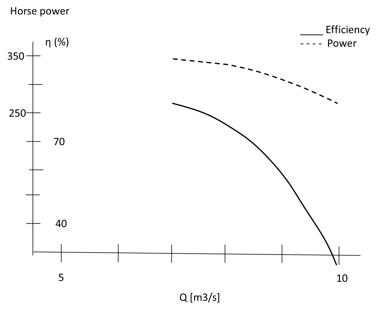
This data is enough to prepare the pump for the optimization.
2. Reading the data
First of all, the data should be read form the pump curves. Since the power curve is available, it is more convenient to read the static head than the manometric head; the static head curve is already corrected for the losses in the system and it is no longer required to determine the head loss Loss h or the head loss coefficient Loss coef.
We read the power from the second graph.
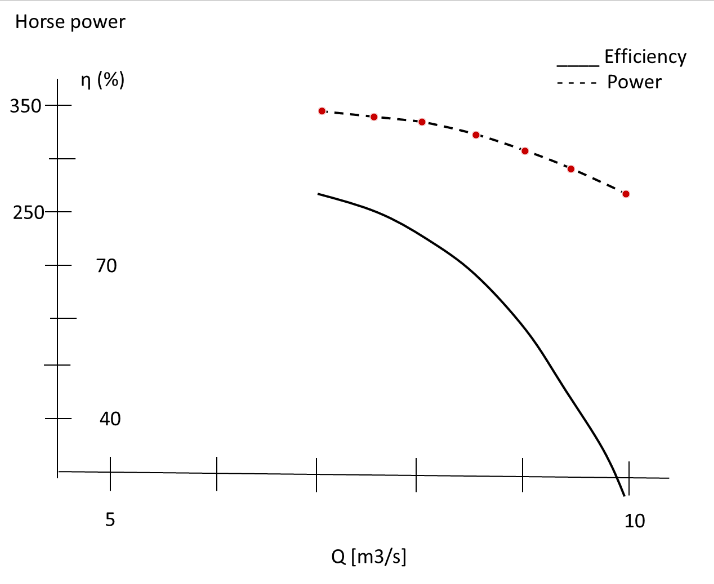
After reading the data it can be organized to the following tables.
| Q (m 3/s) | H(m) |
| 7.8 | 2.2 |
| 8.3 | 1.8 |
| 8.6 | 1.4 |
| 9.0 | 0.9 |
| 9.5 | 0.4 |
| 9.8 | 0.0 |
Note that the power was given in horse power and it should be converted to Watts.
| Q (m 3/s) | P(BHP) | P(W) |
| 7.0 | 346.8 | 255051 |
| 7.5 | 341.6 | 251273 |
| 8.0 | 337.4 | 248154 |
| 8.5 | 325.7 | 239577 |
| 9.0 | 311.2 | 228904 |
| 9.4 | 294.8 | 216836 |
| 10.0 | 271.9 | 200016 |
2. Pre-processing the data
In order to create an input file for the pump fitting tools, every data point should have a Q, H and P value. So the data should be combined to one table by interpolation. In this case the Q values from the first table are kept (as they span a smaller horizon) and the power values are interpolated. Otherwise extrapolation would have been needed which is not recommended.
| Q (m 3/s) | H(m) | P(W) |
| 7.8 | 2.2 | 249400 |
| 8.3 | 1.8 | 243010 |
| 8.6 | 1.4 | 237440 |
| 9.0 | 0.9 | 228900 |
| 9.5 | 0.4 | 214030 |
| 9.8 | 0.0 | 205620 |
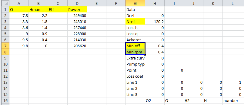
3. Creating the input csv file
The table above should be copied to the csv file. The file should have the give format: 4 columns: discharge, head, efficiency, and power. The headings do not matter but the order of the variables does. The pump speed should be filled in a cell named Nref. There are two more data highlighted in the figure below: the minimum efficiency and the minimum shaft speed for defining the working area of the pump. In other words, what is the minimum efficiency under which the pump should not work. The number should be between 0 and 1. A default value can be 0.4 or 0.5. Same for the minimum shaft speed. Is there a minimum speed under which the pump should not work? Fill in as the fraction of the maximum speed (0-1). 0.4 can be a default value.
No other information is required. Note that the filed Pump type should be zero, as it is a variable speed pump. The csv file should look like this:
4. Running the program
First, the program should know that the data is located in a file Example.csv. It can be done by
editing the file main.py. In the beginning of the file there is a line saying csv_file_name = .
After the equality sign the file name without extension should be typed.
Now the file can actually run by going to the folder src and typing python main.py.
After running the screen should look like:
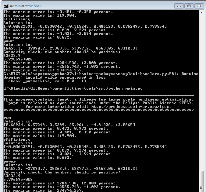
5. Output of the program
The output has several parts, first it says rpm, then efficiency then power. The solution shows six numbers, these are the coefficients of the polynomial fit containing the coefficients of a polynomial
starting with \(c_{1}\). In the following two lines the maximum and minimum error is given (with signs) in absolute value and percentage. Also the maximum value is given to make it easier to judge the errors.
The same type of output is given for the efficiency.
For the power the output is a bit longer. Briefly, the last lines should be read.
The other lines are showing the first approximation attempt of the power. It can be seen that the maximal error is 12 %. If the first attempt is not convex, the program does a second one ensuring convexity. This might result in bigger errors.
These coefficients are also stored in text files in a format suitable to copy them to the
pump model.There are four text files created: power.txt, speed.txt, working_area_fit.txt and efficiency.txt.
The latter is not strictly needed for the pump model.
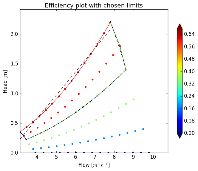
5. Output figures
The plot called EfficiencyWorkingArea shows the calculated efficiency surface and the chosen boundaries of
the working area. The colorful lines are the working area boundaries calculated from the data based on
efficiency and rpm levels. However, they might not be convex. If they are not convex, they are replaced by
convex approximation (black lines).
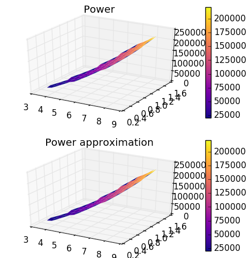
The plot called “surface” shows the original and the approximated power surface.
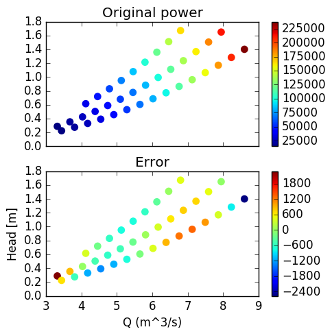
The plot called “powers and error” shows the original power and the error of the power approximation.
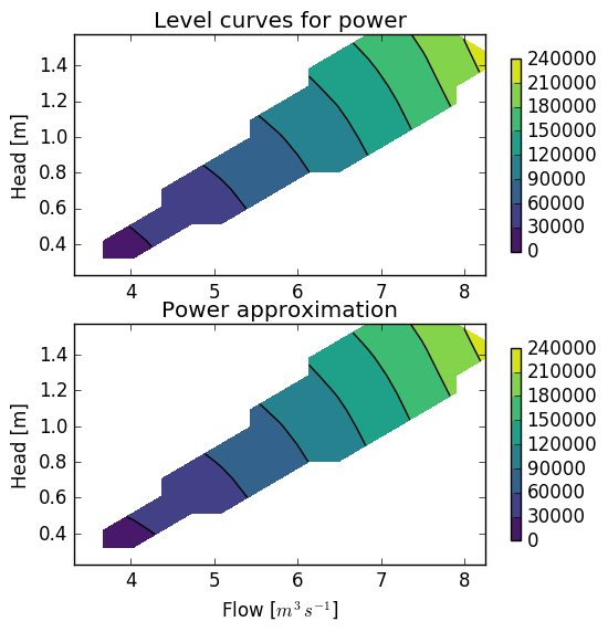
The plot called LevCurvesApprox shows the original and the approximated power as level curves.
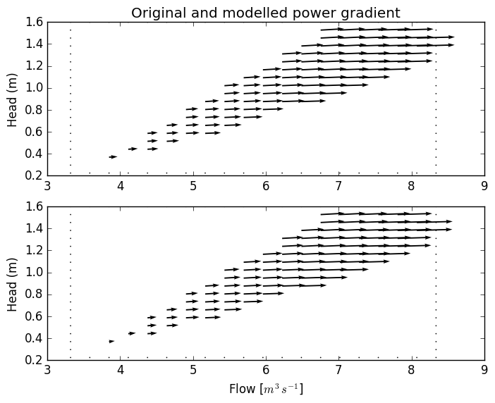
And finally the plot called “Gradients” shows the gradient of the original and approximated power surface. It is important for the optimization that apart from having a small error the gradients also point the same direction.